线性规划
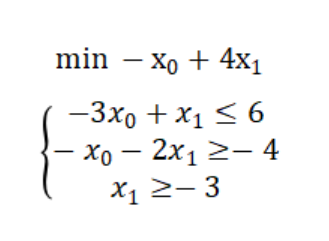
1
2
3
4
5
6
7
8
9
10
11
12
13
14
15
16
17
18
from scipy import optimizeimport numpy as npif __name__ == '__main__' :2 , -3 , 5 ])2 , 5 , -1 ], [1 , 3 , 1 ]])10 , 12 ])1 , 1 , 1 ]])7 ])print (res)
结果:
con: array([1.52631919e-07])
本题是求最大值,那么只需要目标函数加符号,最后将得出的最小值取反即可。
所以本体最大值为14.000000657683216
C = [-1 ,4 ]3 ,1 ],[1 ,2 ]]6 ,4 ]None ,None ],[-3 ,None ]]print (res)
con: array([], dtype=float64)
非线性规划
1 2 3 4 5 6 7 8 9 10 11 12 13 14 15 16 17 18 19 20 21 22 23 24 25 26 27 from scipy.optimize import minimizeimport numpy as npdef fun (args ):lambda x: a / x[0 ] + x[0 ]return vif __name__ == "__main__" :1 ) 2 )) 'SLSQP' )print (res)
计算 (2+x1)/(1+x2) - 3x1+4x3 的最小值, x1, x2, x3 都处于[0.1, 0.9]
区间内。
1 2 3 4 5 6 7 8 9 10 11 12 13 14 15 16 17 18 19 20 21 22 23 24 25 26 27 28 29 def fun (args ):lambda x: (a+x[0 ])/(b+x[1 ]) -c*x[0 ]+d*x[2 ]return vdef con (args ):'type' : 'ineq' , 'fun' : lambda x: x[0 ] - x1min},\'type' : 'ineq' , 'fun' : lambda x: -x[0 ] + x1max},\'type' : 'ineq' , 'fun' : lambda x: x[1 ] - x2min},\'type' : 'ineq' , 'fun' : lambda x: -x[1 ] + x2max},\'type' : 'ineq' , 'fun' : lambda x: x[2 ] - x3min},\'type' : 'ineq' , 'fun' : lambda x: -x[2 ] + x3max})return cons2 ,1 ,3 ,4 ) 0.1 ,0.9 ,0.1 , 0.9 ,0.1 ,0.9 ) 0.5 ,0.5 ,0.5 ))'SLSQP' ,constraints=cons)print (res)
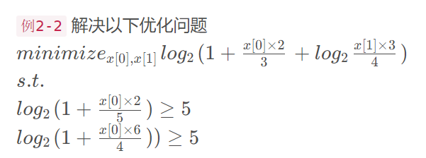
1 2 3 4 5 6 7 8 9 10 11 12 13 14 15 16 17 18 19 20 21 22 23 24 25 26 def fun (a,b,c,d ):def v (x ):return np.log2(1 +x[0 ]*a/b)+np.log2(1 +x[1 ]*c/d)return vdef con (a,b,i ):def v (x ):return np.log2(1 + x[i] * a / b)-5 return v2 , 1 , 3 , 4 ] 2 , 5 , 6 , 4 ] 0.5 , 0.5 ))'type' : 'ineq' , 'fun' : con(args1[0 ],args1[1 ],0 )},'type' : 'ineq' , 'fun' : con(args1[2 ],args1[3 ],1 )},0 ], args[1 ], args[2 ], args[3 ]), x0, constraints=cons)print (res)
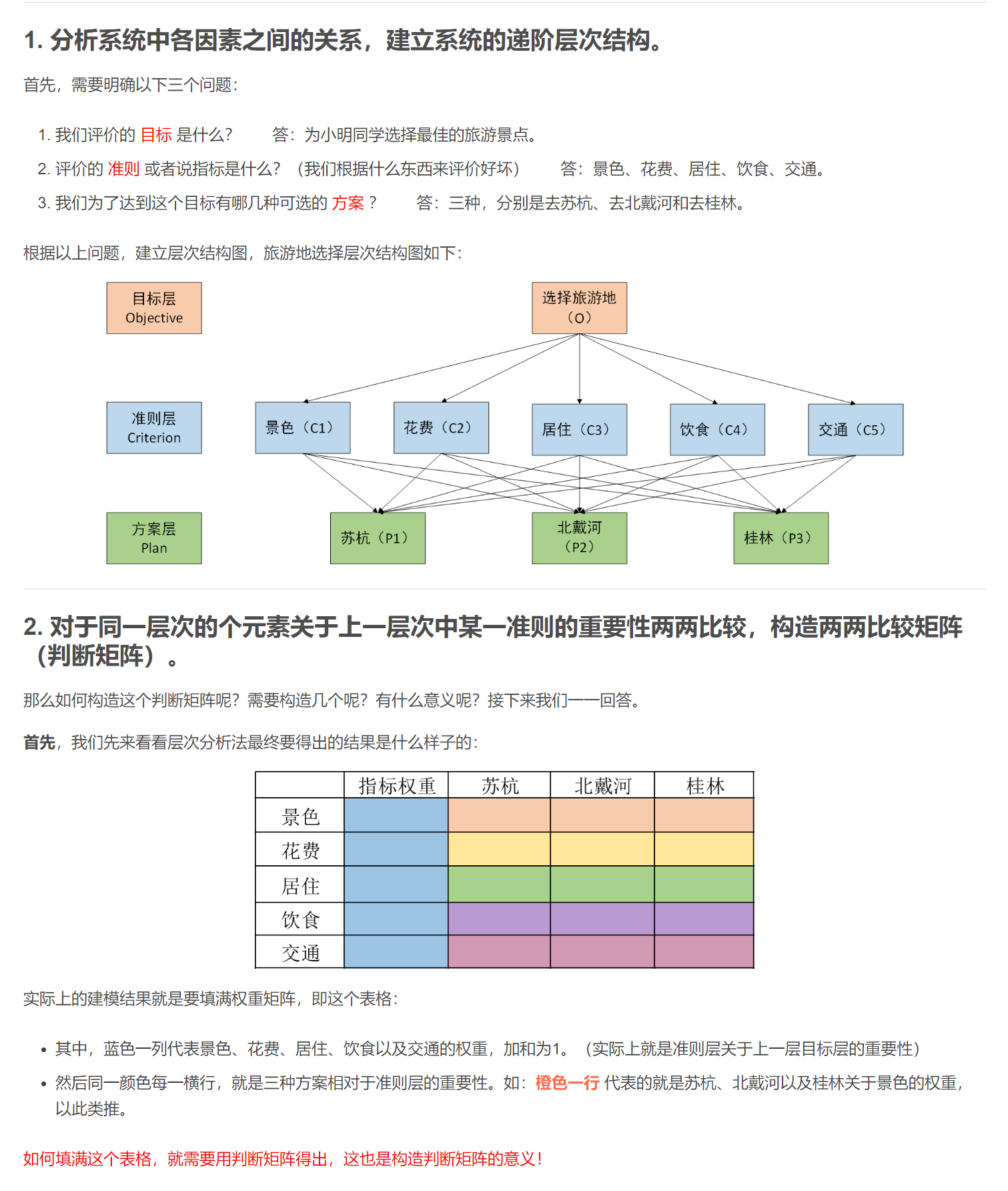
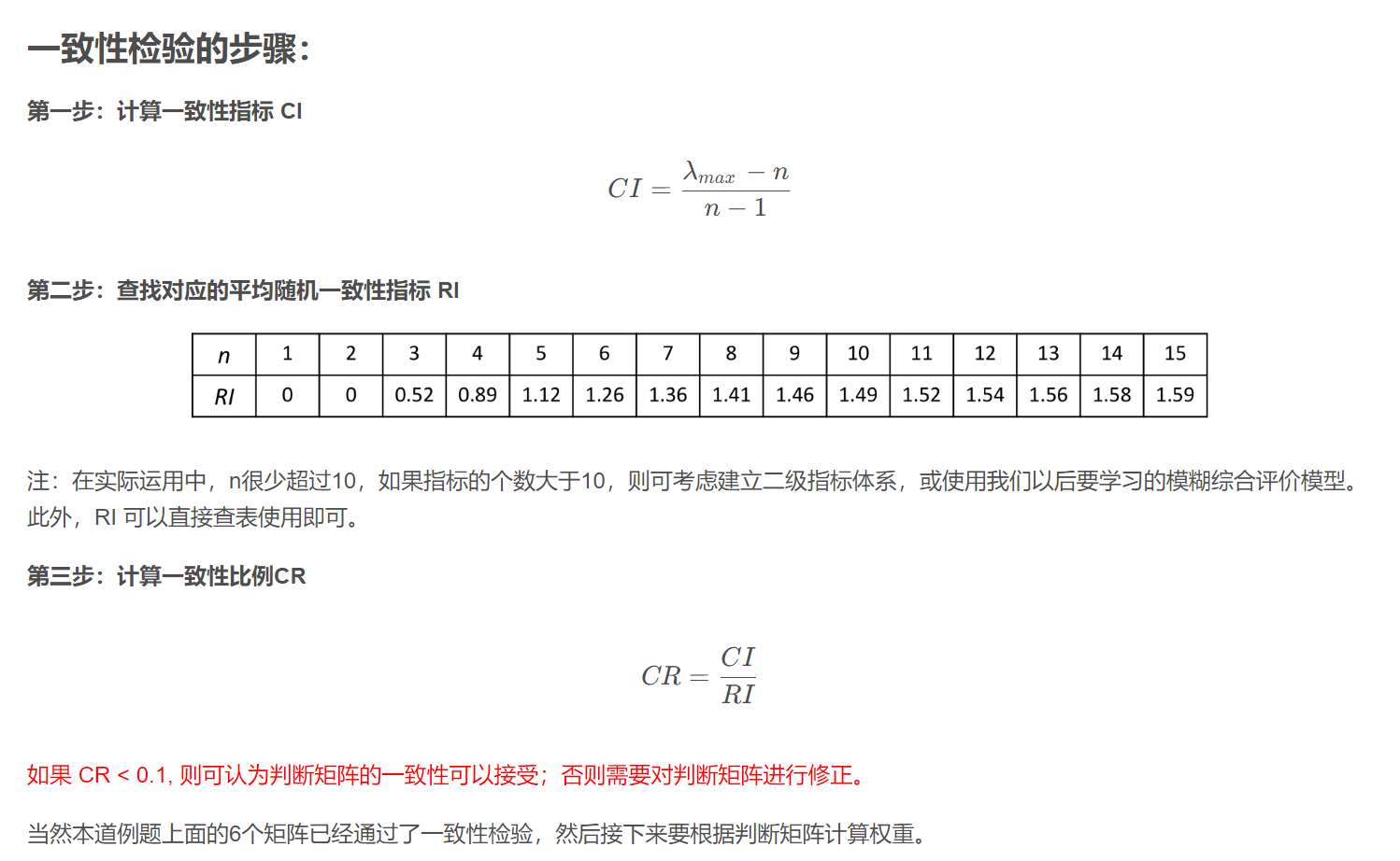
层次分析法
https://blog.csdn.net/weixin_43819566/article/details/112251317
Topsis(优劣解距离法)
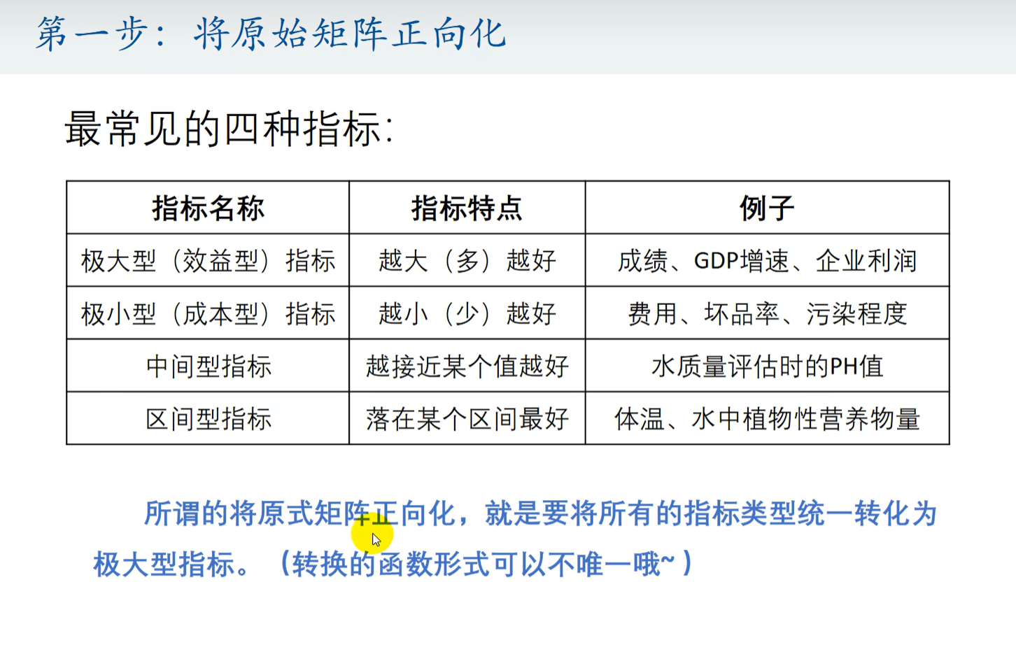
第一步 将指标正向化
第二步 将指标归一化
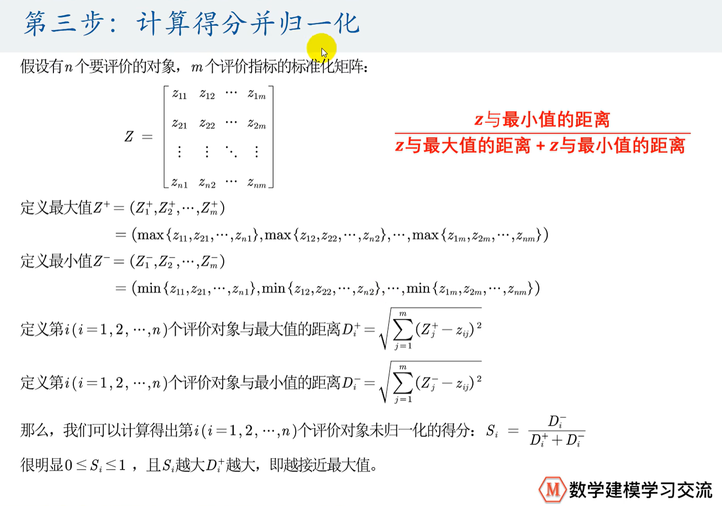
第三步 计算得分并归一化
代码实现
https://blog.csdn.net/weixin_52300428/article/details/126309794
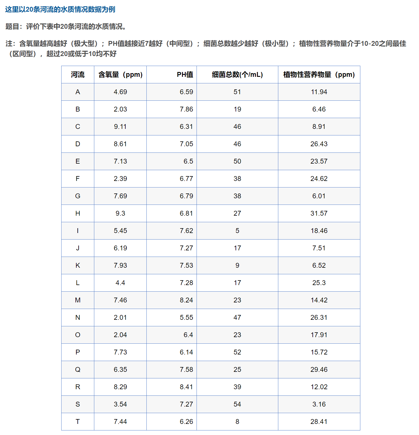
1 2 3 4 5 6 7 8 9 10 11 12 13 14 15 16 17 18 19 20 21 22 23 24 25 26 27 28 29 30 31 32 33 34 35 36 37 38 39 40 41 42 43 44 45 46 47 48 49 50 51 52 53 54 55 56 57 58 59 60 61 62 63 64 65 66 67 68 69 70 71 import pandas as pdimport numpy as npdef Mintomax (datas ):return np.max (datas) - datasdef Midtomax (datas, x_best ):max (abs (temp_datas))1 - abs (datas - x_best) / Mreturn answer_datasdef Intertomax (datas, x_min, x_max ):max (x_min - np.min (datas), np.max (datas) - x_max)for i in datas:if (i < x_min):1 - (x_min - i) / M)elif (i > x_max):1 - (i - x_max) / M)else :1 )return np.array(answer_list)def Standard (datas ):sum (pow (datas, 2 ), axis=0 ), 0.5 )for i in range (len (k)):return datasdef Score (sta_data ):0 )0 )sum (np.power((z_max - sta_data), 2 ), axis=1 ), 0.5 )sum (np.power((z_min - sta_data), 2 ), axis=1 ), 0.5 )sum (score) return scoreif __name__ == '__main__' :r'./20条河流的水质情况数据.xlsx' )'细菌总数(个/mL)' ] = Mintomax(df['细菌总数(个/mL)' ]) 'PH值' ] = Midtomax(df['PH值' ], 7 ) '植物性营养物量(ppm)' ] = Intertomax(df['植物性营养物量(ppm)' ], 10 , 20 ) 1 :]'score' ] = sco'Topsis.csv' , index=False , encoding='utf_8_sig' )
分类
1 2 3 4 5 6 7 8 9 10 11 12 13 14 15 16 17 18 19 20 21 22 23 24 25 26 27 28 from sklearn.linear_model import LogisticRegressionfrom sklearn.metrics import accuracy_scorefrom sklearn.model_selection import train_test_splitfrom sklearn.svm import LinearSVC, SVCfrom sklearn.preprocessing import StandardScaler0.3 )"linear" , "poly" , "rbf" , "sigmoid" ]"rbf" )
回归
1
2
3
4
5
6
7
8
9
10
11
12
13
14
15
16
17
18
19
20
21
22
23
24
25
26
27
import numpy as npfrom sklearn.linear_model import LinearRegression, Lasso, Ridgeimport matplotlib.pyplot as plt"data.csv" , delimiter="," )0 :-1 ]1 ]102 , 4 ]]0.1 )0.1 )